S&S_Forecasts - Center for Western Weather and Water Extremes

A multi-institutional collaboration sponsored by California DWR

Subseasonal and Seasonal (S&S) Experimental Forecasts

Subseasonal Forecasts (Weeks 1-6)

Click here to view the latest CW3E Subseasonal Outlook

– Archive of previous S&S Outlooks

Dynamical Model Atmospheric River Activity Forecasts

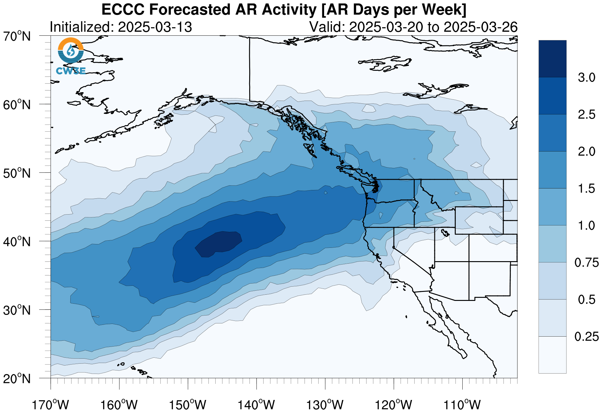
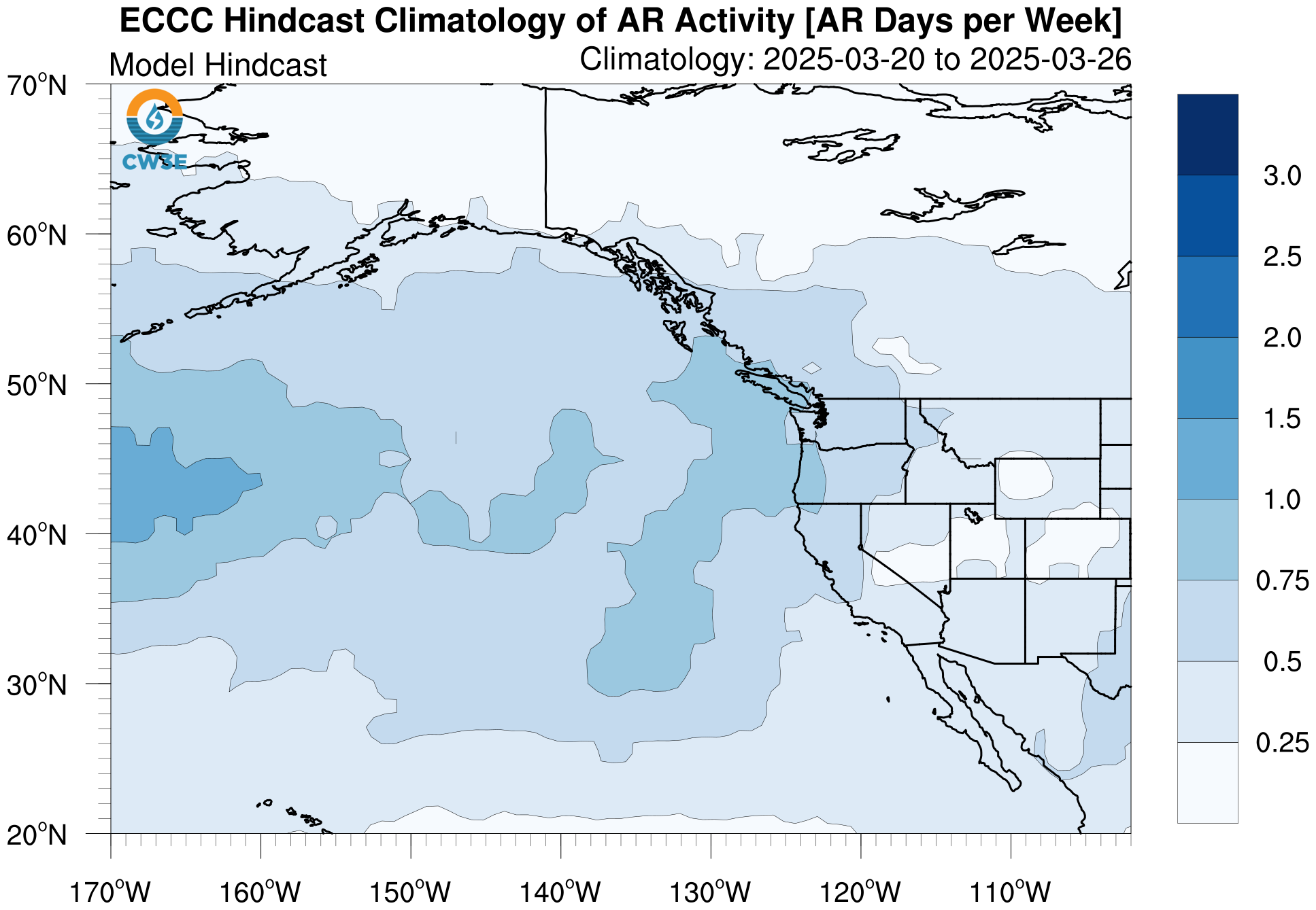
A multi-model experimental forecast for AR activity (defined as the # of AR days per week) at week-2, 3, and 4 lead time is shown below for the NCEP, ECMWF, ECCC, and NASA GMAO dynamical models.

Top left: Forecasted number of AR days per week. Top right: Climatological values of AR activity in each model’s hindcast record for the corresponding lead time verification period. Bottom row: Departure from normal of the AR activity forecast (top left minus to right) shown in AR days per week (bottom left) and percentage anomaly (bottom right). Areas of green (brown) represent higher (lower) than average AR activity predicted during the selected week. The hindcast skill assessments associated with these dynamical model hindcast systems are described in both DeFlorio et al. 2019b and Zhang et al. 2023.
NOTE: models will not always be initialized on the same day. Please check the initialization date in the title of the plots.

Model:

Lead Time:

Region:

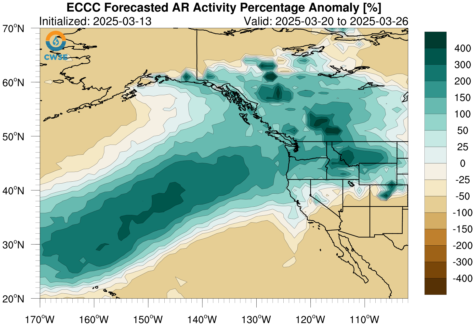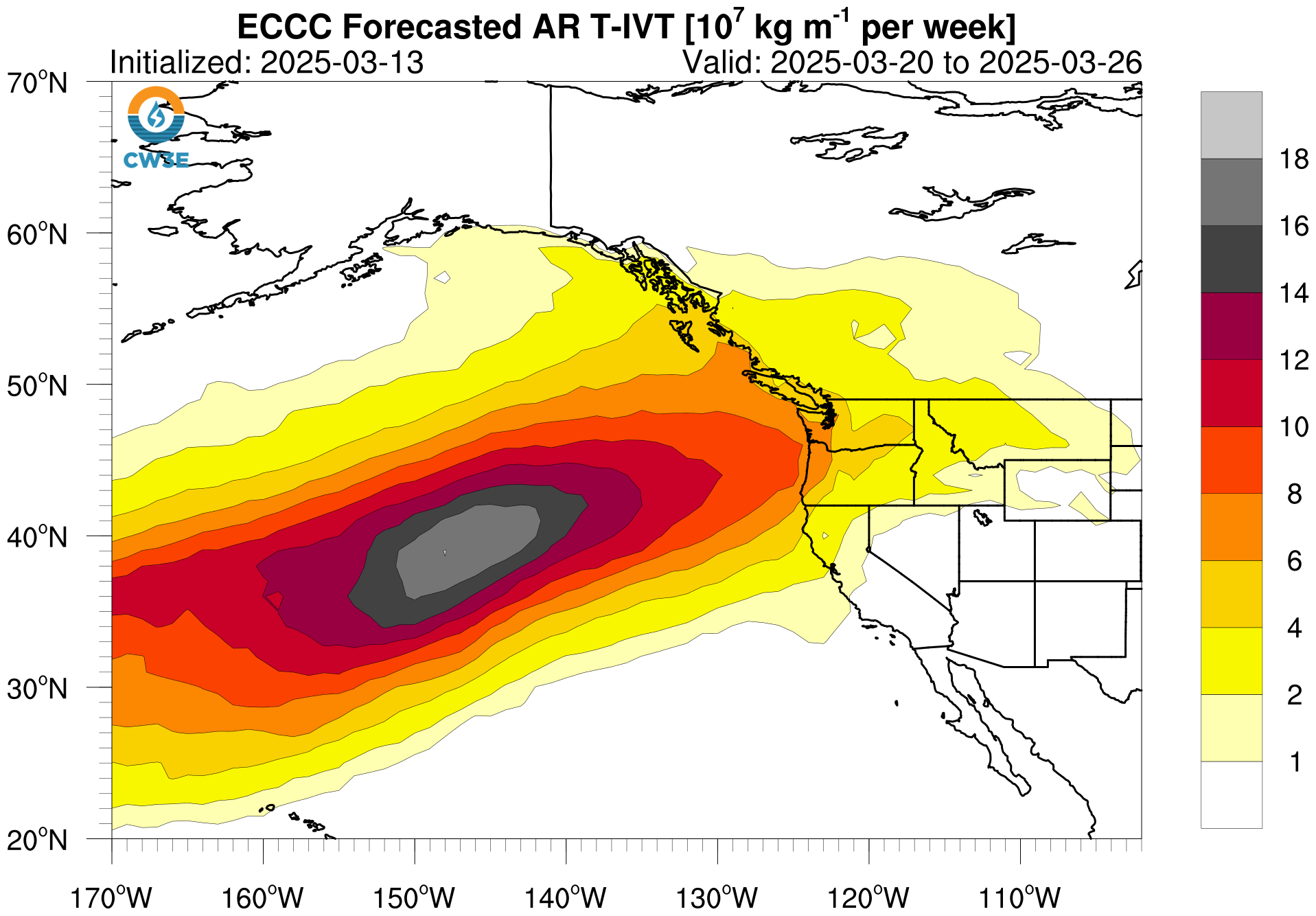
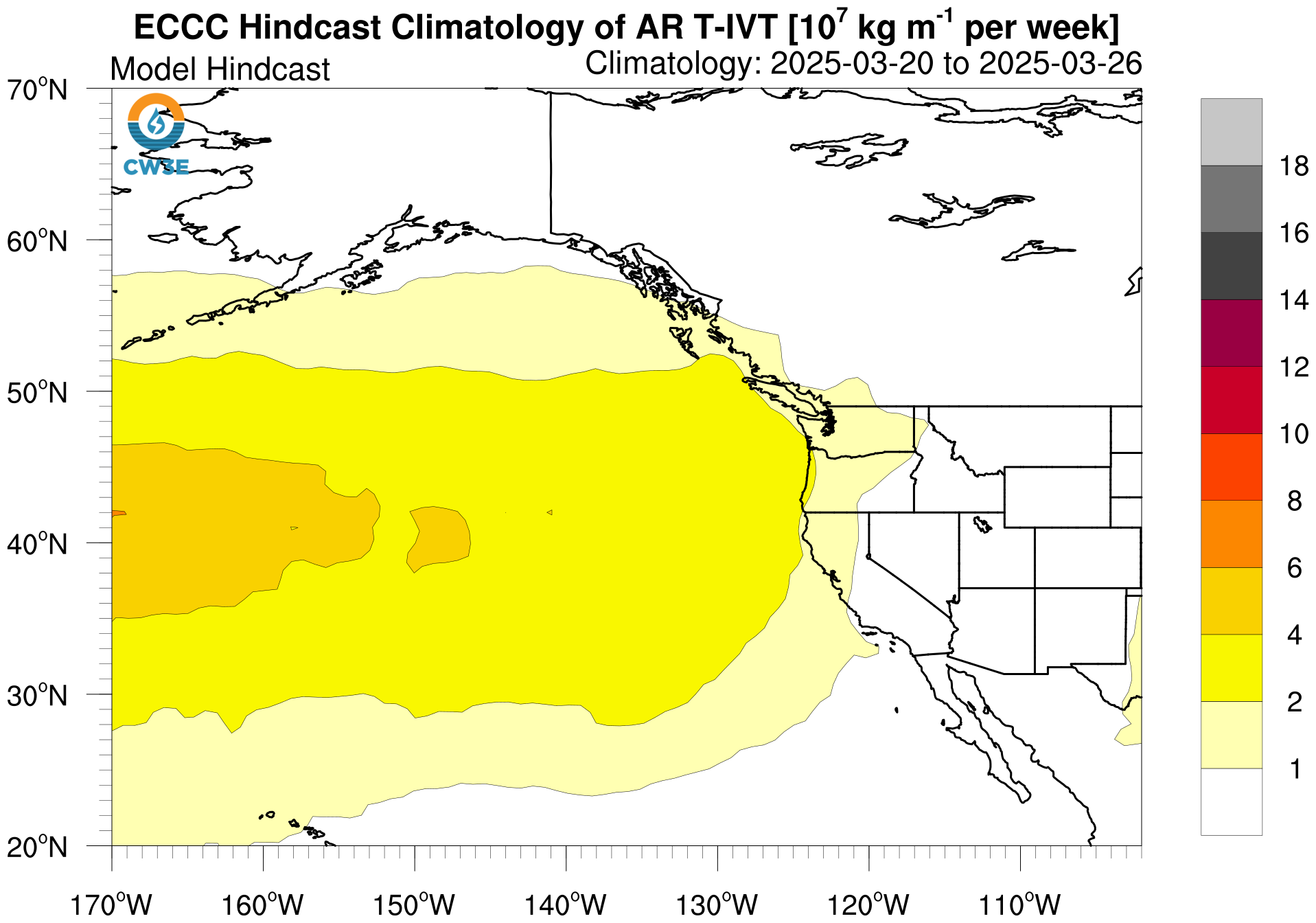
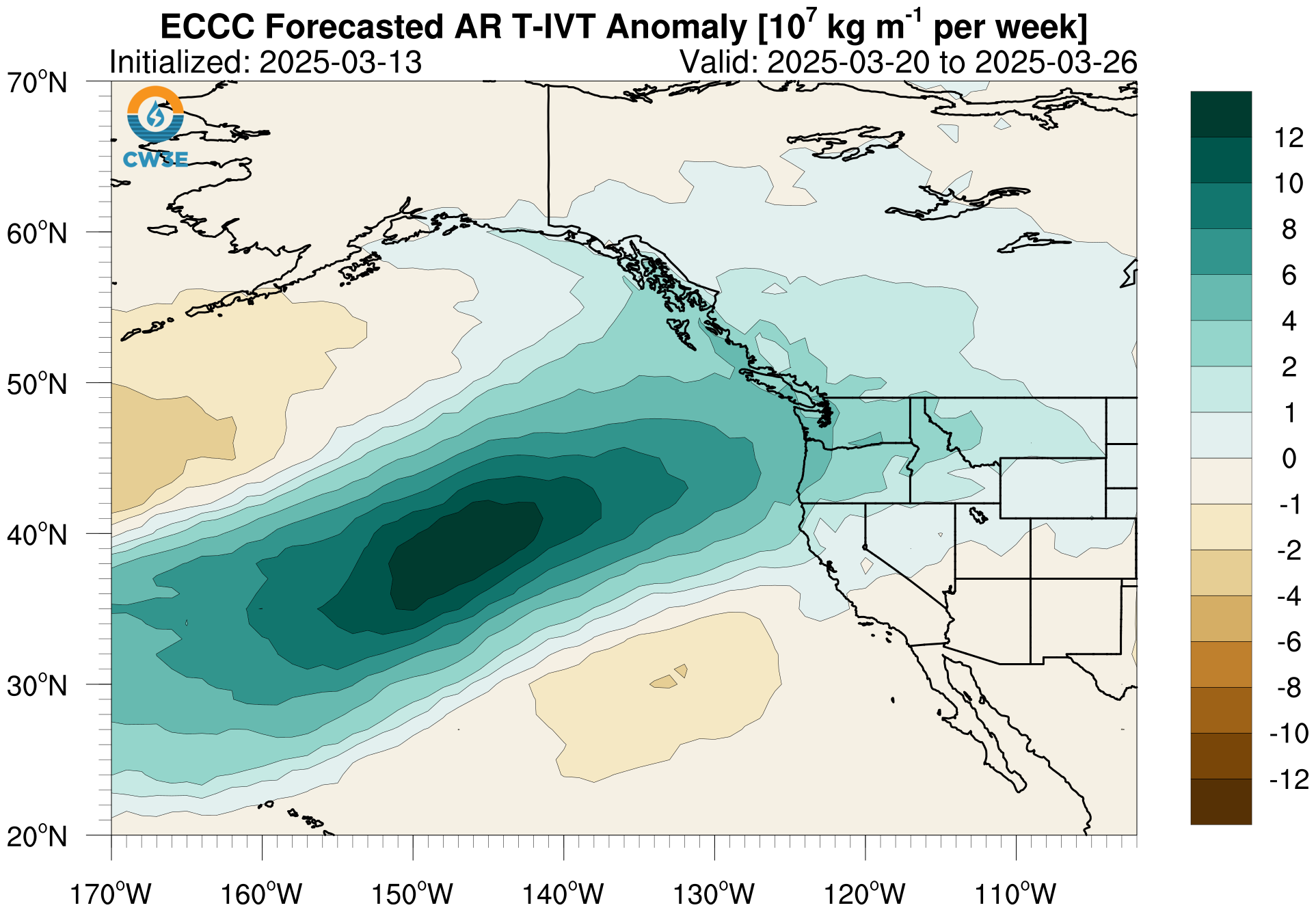
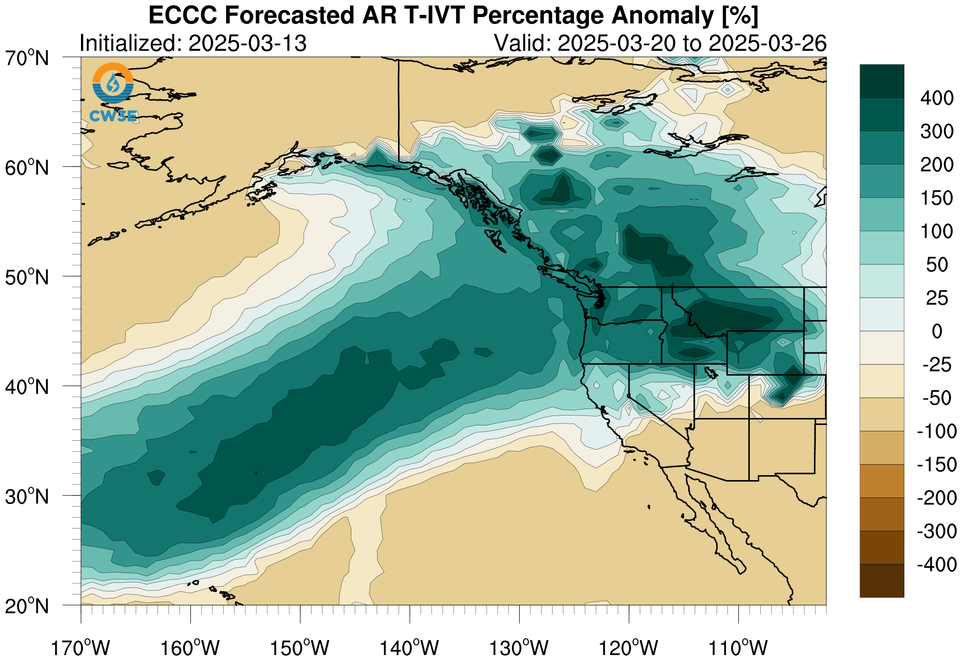
Dynamical Model Atmospheric River Intensity Forecasts

A multi-model experimental forecast for AR intensity (defined as the AR related time-integrated water vapor transport (TIVT)) at week-2, 3, and 4 lead time is shown below for the NCEP, ECMWF, ECCC, and NASA GMAO dynamical models.

Top left: Forecasted AR related time-integrated water vapor transport (TIVT; 10⁷ kg m^-1) per week. Top right: Climatological values of AR-related TIVT in each model’s hindcast record for the corresponding lead time verification period. Bottom row: Departure from normal of the TIVT forecast (top left minus to right) shown in TIVT per week (bottom left) and percentage anomaly (bottom right). Areas of green (brown) represent higher (lower) than average TIVT predicted during the selected week. The hindcast skill assessments associated with these dynamical model hindcast systems are described in both DeFlorio et al. 2019b and Zhang et al. 2023.
NOTE: models will not always be initialized on the same day. Please check the initialization date in the title of the plots.

Model:

Lead Time:

Region:

Atmospheric River Activity and Intensity Forecast for Week-3

The number of days with forecasted AR conditions in week-3 at various locations over the western U.S. from the NCEP, ECMWF, GAMO, and ECCC dynamical models. ARs are classified by intensity based on the AR strength scale from Ralph et al. 2019 (Weak: IVT < 500 kg m^-1 s^-1, Moderate: 500 > IVT > 750 kg m^-1 s^-1, Strong: 750 > IVT > 1000 m^-1 s^-1, Extreme: 1000 > IVT > 1250 m^-1 s^-1, and Exceptional: IVT > 1250 m^-1 s^-1) for each ensemble member and the ensemble mean (EM). Ensemble spread in the total number of AR days (All AR) is shown in the box and whisker plot. The climatology of the total number of AR days for this week is represented by the dashed black line.
NOTE: models will not always be initialized on the same day. Please check the initialization date in the title of the plots.

Model:

Lead Time:

Location:

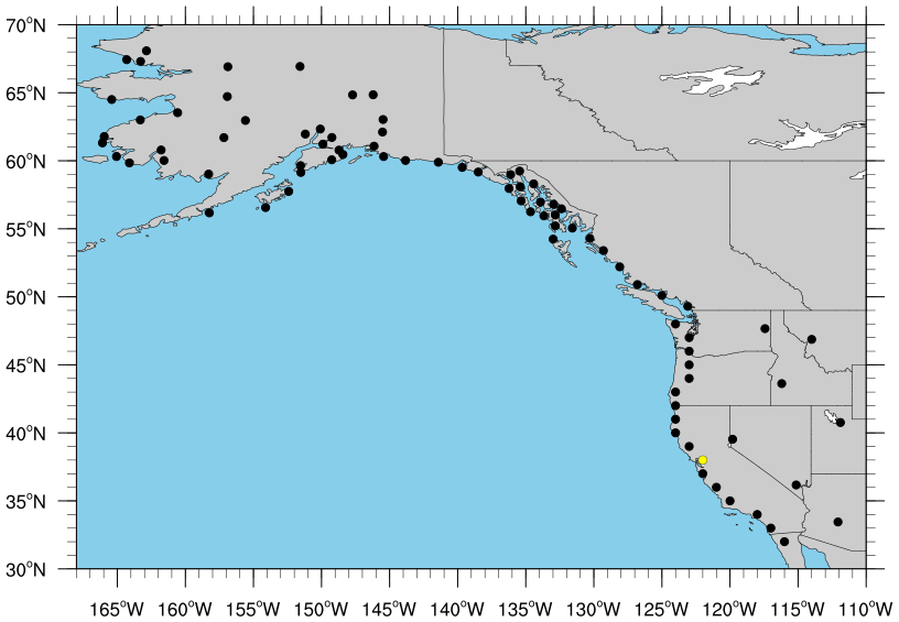
Atmospheric River IVT Forecast for Week-3

The time-integrated IVT (kg m^-1) in week-3 at various locations over the western U.S. from the NCEP, ECMWF, and ECCC dynamical models. IVT associated with an AR (AR IVT, red bars) and IVT not associated with an AR (NO-AR IVT, blue bars) are plotted for each ensemble member and the ensemble mean (EM). Ensemble spreads in total IVT (All IVT) and AR IVT are shown in the box and whisker plots. The climatology of total IVT and AR IVT for this week is represented by the dashed black line and red line respectively.
NOTE: models will not always be initialized on the same day. Please check the initialization date in the title of the plots.

Model:

Lead Time:

Location:

Dynamical Model Subseasonal Ridging Forecasts

An atmospheric ridge is defined as elongated area of relatively high atmospheric pressure (American Meteorological Society; 2020). Persistent ridging events play an important role in determining if and where precipitation falls. Ridging forecasts are shown below for lead-times of weeks 1 and 2, weeks 3 and 4 and weeks 5 and 6. These forecasts are for three different ‘ridge types’ that have been shown in recent research [Gibson et al. 2020a; more methodology information here] to strongly influence atmospheric river and precipitation likelihood across the US West Coast. The North-ridge type is typically associated with widespread dry conditions across the entire US West. The South and West-ridge types are typically associated with dry conditions across Southern California and the Colorado River Basin but can also increase the likelihood of wet conditions across the Pacific Northwest. The hindcast skill assessment associated with this outlook is provided in Gibson et al. 2020b.

This product was developed in collaboration with NASA’s Jet Propulsion Laboratory.

This product was designed and has been tested only during the winter months, this product will be produced and available again in early October 2025.

Subseasonal Forecast of North American Weather Regimes

Forecast from IRI.

The graphic shows forecasts of large scale meteorological patterns, issued every day during winter (along x-axis) by the NCEP CFSv2 model. The four large scale “weather regimes” are the West Coast Ridge (reds), Pacific Ridge (blues), Pacific Trough (greens), and Greenland High (yellows), each of which leads to distinct precipitation and temperature conditions over the West. Darker colors indicate more confident forecasts, which run diagonally up the chart from 0 to 45 days ahead. This product was developed with support from NOAA’s Next Generation Global Prediction System (NGGPS) program and the California Department of Water Resources. Please see https://wiki.iri.columbia.edu/index.php?n=Climate.S2S-WRs for the precipitation and temperature signatures of the regimes or Robertson, Vigaud, Yuan & Tippett (2020) for additional details.

This product is run from October – March, an updated forecast will be available on October 1, 2025.

Subseasonal AR Activity and Precipitation Outlooks Based on MJO and QBO

This product shows weekly probabilities of above-normal and below-normal AR activity and precipitation in California. These probabilities are calculated for lead times of 1–6 weeks based on the current season (i.e., OND or JFM) and phases of the Madden-Julian Oscillation (MJO) and Quasi-biennial Oscillation (QBO). The user must select a region (Northern California, Central California, or Southern California) and a variable (AR occurrence, AR-TIVT, or precipitation) to display. AR occurrence is defined as the number of hours with AR conditions during a 7-day period in the selected region (blue rectangles on inset map). AR-TIVT is defined as the time-integrated IVT associated with ARs during a 7-day period in the selected region (blue rectangles on inset map). Precipitation is defined as the mean areal precipitation during a 7-day period in the selected region (red outlines on inset map). If MJO convection is weak or the QBO is in a neutral phase, no probabilities will be displayed. The MJO is considered “weak” when the real-time multivariate MJO index (Wheeler and Hendon 2004) is < 1. The QBO is considered “neutral” when the absolute value of the 50-hPa standardized monthly zonal wind index is < 0.5. Daily MJO data and monthly QBO data are provided by the Climate Prediction Center.

This product was designed and has been tested only during the winter months, this product will be produced and available again in early October 2025.

Seasonal Forecasts (1-3 months)

CW3E Seasonal forecast products are updated twice during the water year: once in mid-November and once in January. The latest CW3E seasonal forecasts can be found in the most recent Seasonal Outlook.

Click here to view the latest CW3E Seasonal Outlook

– Archive of previous S&S Outlooks

CCA 3-Month Precipitation Forecasts

The forecasting method predicts three month accumulated precipitation using a statistical method based on canonical correlation analysis (CCA) to identify temporally coupled and physically meaningful spatial modes in sea surface temperature and precipitation. This approach uses December 2024 observed monthly Pacific sea surface temperature anomalies to predict accumulated precipitation amounts during January – March 2025 based on historical relationships. The left plot show the accumulated precipitation relative anomalies and the right plot show historical skill for this forecast. Skill is defined as the correlation coefficient between the time series of observed and predicted seasonal precipitation at each grid cell using "leave-one-out" cross-validation iteration over each three month period 1948-2015 and December SST forcing. For more information on this method click here. The hindcast skill assessment for these products is available in Gershunov and Cayan 2003.

CW3E Seasonal forecast products are updated twice during the water year: once in mid-November and once in January. An updated version of this product will be available in early November.

Seasonal Precipitation Forecast based on a Machine Learning Approach

This CW3E forecast product predicts likely seasonal precipitation anomaly patterns for January-February-March over the western U.S. based on machine learning models and dynamical ensemble predictions. Four different machine learning models (Random Forest, XGBoost, LSTM, and neural networks) were pretrained based on learning relationships between remote ocean and atmospheric patterns and characteristic seasonal precipitation anomalies over the Western United States. Instead of training on observations, the machine learning models were here trained on a large climate model ensemble, which enabled more robust relationships to be established due to the very large sample size in the training phase (Gibson et al. 2021). Seasonal forecast skill is also enhanced by focusing on four characteristic large-scale precipitation patterns across the Western United States. Our historical skill assessment found that the probability of a correct forecast improves when the Machine learning models show stronger consensus for a particular pattern. As such, the ensemble agreement (or lack of) provides useful guidance on forecast uncertainty.

This product was developed in collaboration with NASA’s Jet Propulsion Laboratory.

CW3E Seasonal forecast products are updated twice during the water year: once in mid-November and once in January. An updated version of this product will be available in early November.

University of Arizona Seasonal Temperature, Precipitation, and Snowpack Forecasts

The University of Arizona team (Bill Scheftic and Xubin Zeng) uses the ensemble seasonal predictions from NCEP and ECMWF with two-stage revisions for our seasonal prediction of NDJ 2-m temperature (T2m), precipitation (P), and snow water equivalent (SWE) over the western U.S. The first stage performs a bias correction, while the second stage makes use of climatological indexes to further improve the prediction. The two adjusted model forecasts are combined with two empirical approaches to create our seasonal forecast. The method and the historical performance of our method are discussed in more detail in Scheftic et al. (2023, 2024).

CW3E Seasonal forecast products are updated twice during the water year: once in mid-November and once in January. An updated version of this product will be available in early November.

Six-Month Seamless Forecast of North American Weather Regimes

Forecast from IRI.

The winter seamless forecasts show the forecasts for the full range October 1, 2024 — March 31, 2025, updated every day. They use the lead-time averaging ranges on the ordinate that widen with lead time: days 2-3, days 4-7, week 2, weeks 3-4, followed by monthly-averaged forecasts from month 2 to month 6. The month boundaries are indicated by horizontal blue lines. The lead-time averaged forecast anomalies were computed prior to projection on the MERRA regime patterns. Please see https://wiki.iri.columbia.edu/index.php?n=Climate.S2S-WRs for the precipitation and temperature signatures of the regimes or Robertson, Vigaud, Yuan & Tippett (2020) for additional details.

This product is run from October – March, an updated forecast will be available on October 1, 2025.

For additional products and more information visit the Odds of Reaching 100% of Normal Water Year Precipitation webpage.

All products displayed on this page are considered experimental.